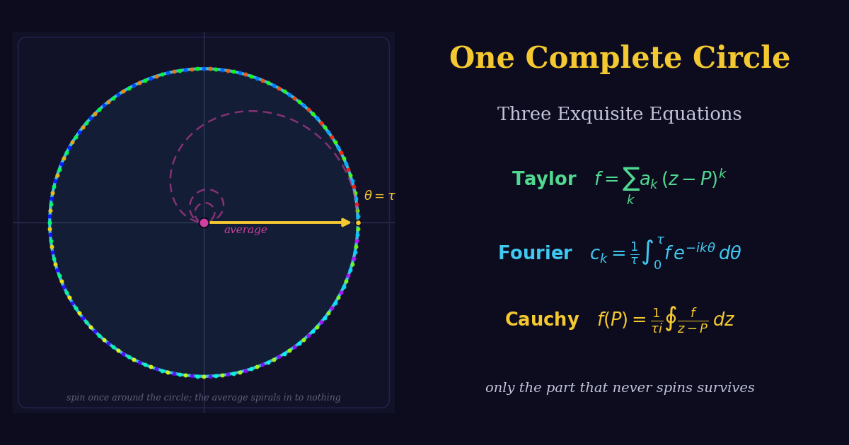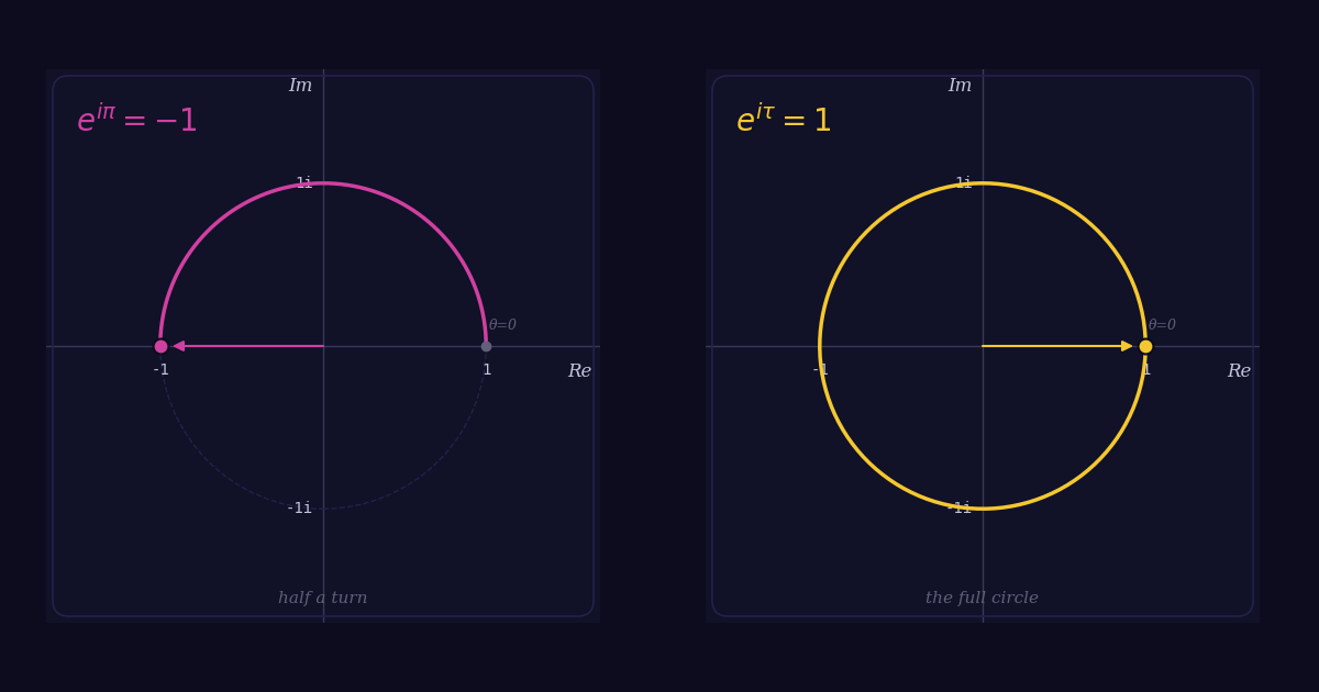
The Natural Occurrence of x²2
Part 1 — Why is v = t the natural velocity?
Gravity is a familiar example of constant acceleration — near Earth's surface it accelerates falling objects at ≈ 9.8 m/s² downward, almost perfectly constant over human scales. Acceleration is the rate at which velocity changes:
a = dvdtRearranging: each tiny slice of time dt delivers a velocity push dv = a · dt. Setting a = 1 normalises the numbers without changing the structure. With a = 1: dv = dt.
Now see how a constant a builds v across the same time horizon:
Left — constant a = 1 across time. N colored blocks, each with height 1 and width dt, and therefore area:
1 · dt = a · dt = dt = dvRight — v across time. Across each time interval, v grows by dv by definition: each tick length on the right corresponds to the area of a block on the left, fitting well to v = t at large N. Drag N:
Constant acceleration g = 1 — each colored block is one velocity increment dv = g · dt
Colored ticks are lengths dv — stacking them on the velocity axis gives v = Σ dv = t
As N → ∞, each slice gets thinner and the staircase becomes the smooth line v = t. That line is not chosen — it is forced on us by the constancy of gravity: equal pushes accumulate into linear growth.
Part 2 — Why is x = t²/2 the natural distance?
Distance is velocity times time. Each instant contributes a thin strip of area v · dt = t · dt, and total distance is the sum of all strips — the area under v = t.
That region is a right triangle with base t and height t. Its area is exactly half the enclosing square:
x = ½ · t · t = t²2Left — v = t across time. Each colored strip has height v and width dt, and therefore area:
v · dt = t · dt = dxRight — distance x(t) across time. At each moment the distance grows by the area of the strip on the left: each tick length on the right equals one strip's area, tracing out x(t) = t²/2 at large N. Drag t — or play to animate:
Each colored strip has area = distance increment dx = v · dt
Same strips stacked as tick lengths — staircase traces x(t) = t²/2
The parabola t²/2 on the right is the growing triangle on the left. Its slope at any point recovers the velocity: d/dt (t²/2) = t. The line and the parabola are each other's mirrors.
Key insight. t²/2 is the natural distance because it is the area of the triangle formed by linear velocity — and the area of any triangle is half its enclosing square. The ½ comes from geometry, not convention.
Part 3 — x²/2 appears wherever something grows linearly
Part 2 showed that distance under constant acceleration is t²/2. That result is an instance of a deeper pattern. The reason it appeared is simple:
ddx (x²2) = xx²/2 is the integral of x — the natural accumulation of anything that grows proportionally to x itself. Whenever physics gives you a quantity that increases linearly, integrating it produces x²/2. The ½ is not inserted by hand; it is the area of the triangle between the line and the axis.
Two more examples from physics — both familiar, both the same triangle:
Kinetic energy. A force F = ma accelerates a mass. Velocity grows linearly in time: v = at. Work = force × distance, and distance = t²/2 from Part 2. So:
KE = 12mv²The ½ is the same triangle from Part 2 — velocity built linearly from 0, so the average is half the final value.
Spring energy. Hooke's law says the restoring force grows proportionally to displacement: F = kx. The work to compress the spring by x is the area under that line — another triangle:
PE = 12kx²Key insight. ½mv² and ½kx² both carry a ½ for the same reason: the physical quantity (velocity, force) grows linearly, so its accumulated effect is the area of a triangle — exactly half the enclosing rectangle. x²/2 is the universal signature of linear growth integrated once.
The Natural Occurrence of 1/x, log(x) and exp(y)
Part 1 — Why does 1/x arise naturally?
Boyle's law is a familiar example of an inverse relationship — hold temperature fixed, and pressure and volume are inversely linked. Setting the proportionality constant to 1:
PV = 1 ⟹ P = 1VHalve the volume: pressure doubles. Compress to a third: pressure triples. Plotted against volume, this is the curve y = 1/x.
Now ask: how much work does expanding the gas from volume 1 to volume V release? Work is pressure times volume change. Each tiny expansion dV contributes:
dW = P · dV = 1V dVLeft — pressure P = 1/V across volume. N colored blocks, each with height 1/V and width dV, and therefore area:
1V · dV = P · dV = dWRight — work W across volume. Each tick length on the right corresponds to the area of a block on the left, stacking toward W = log V at large N. Drag N to refine; drag V to extend — or play:
Each colored rectangle has area = work contribution dW = (1/V)·ΔV
Same rectangles stacked as heights — the staircase approximates W = log V
As N → ∞ the staircase fills the smooth gold curve. That curve — the accumulated area under 1/V — is the logarithm. It is one of the most important functions in mathematics and science: the natural language of anything that grows or shrinks by ratios rather than by fixed amounts.
Part 2 — Equal ratios, equal areas
Drag V past 2, then past 4 in the charts above. Each doubling adds exactly the same height to the right chart — the intervals 1→2, 2→4, and 4→8 all contribute identical work, log 2 ≈ 0.693, regardless of where on the axis they sit:
Three doublings of volume — each shaded region is the same work, log 2
Here is why: dV/V measures relative change, and relative change is blind to scaling. Replace V with c · V everywhere — the strip becomes d(c·V) = c · dV wide, the height becomes 1/(c·V), and the c cancels:
d(c · V)c · V = c · dVc · V = dVVBoth strips have the same area dV/V — the 1/(c·V) height and the c·dV width cancel exactly
Key insight. Musical pitch works exactly this way. The step 220 Hz → 440 Hz and the step 440 Hz → 880 Hz feel identical — both are an octave. The absolute widths are 220 Hz and 440 Hz; the ratio is 2 in both cases. Our ears integrate df/f, not df. The 1/f weighting makes the integrand scale-invariant, so only the ratio between the startpoint and endpoint is heard.
Part 3 — log: converting multiplication to addition
Scaling the interval by a constant c leaves the integrand unchanged — the result depends only on the ratio Ve/Vs, wherever the interval sits.
Now ask: what happens to relative change when two varying quantities are multiplied? The relative change in a product x · y is d(xy) and its inverse is 1/(xy).
Let's first look at d(xy). The diagram shows what it is. Expanding the new rectangle gives four pieces: the original xy, two thin strips y·dx and x·dy, and a tiny corner dx·dy. The last term is the product of two small quantities — as dx, dy → 0, it vanishes, leaving the exact relation above.
d(xy) = (x + dx)(y + dy) — xy = y·dx + x·dy, as the shaded corner dx·dy vanishes as the steps shrink
d(xy) = y dx + x dy and divide by xy:
d(xy)xy = dxx + dyyRelative changes approximately add. Say x = 100, dx = 3, y = 80, dy = 1.6. Then dx/x and dy/y represent their respective relative changes in the familiar sense: dx/x = 3% and dy/y = 2%. A 3% rise in x and a 2% rise in y produce a 5.06% rise in xy — not exactly 5%, because the corner dx · dy = 0.03 × 0.02 = 0.06% is small but nonzero. As the steps shrink toward zero the corner vanishes, and the approximation becomes exact.
We saw earlier in Part 1 that log is used to show the accumulation of infinitesimal relative steps of dt/t. So log(xy) is simply the total of all the small changes d(log(xy)) as xy grows from 1 to its final value, and each such step is d(log(xy)) = d(xy)/(xy).
Exactly the same is true term by term: log(x) is the sum of all d(log x) = dx/x, and log(y) is the sum of all d(log y) = dy/y. Since each set of infinitesimal pieces satisfies d(xy)/(xy) = dx/x + dy/y exactly, so does their total — we get an equation in aggregation:
log(a · b) = log(a) + log(b)Not a definition — a consequence. The logarithm converts multiplication into addition because 1/x measures relative change, and relative changes add.
Part 4 — exp: converting addition to multiplication
exp is the inverse of log. Where log converts multiplication into addition, exp goes the other direction — it converts addition back into multiplication:
exp(a + b) = exp(a) · exp(b)Graphically, the two functions are exact reflections of each other across the diagonal y = x. Every point (x, log x) on the log curve has a mirror (log x, x) on the exp curve — coordinates swapped. Two sample mirror pairs are marked:
log x and exp x are mirror images across y = x
One famous property of exp falls out of this mirror picture almost for free: exp is its own derivative. The argument is purely geometric — and traces straight back to 1/x.
First, the slope of log. By Part 1, log x = ∫₁ˣ dt/t — the accumulated area under 1/t from 1 to x. How fast does this area grow as x increases? When the right edge advances from x to x + dx, the area gains a thin vertical strip of width dx and height 1/x — the value of the integrand at that edge. So the added area is (1/x) · dx, and the rate of growth is simply the height 1/x:
ddx log(x) = 1xThis is the fundamental theorem of calculus in its most geometric form: the derivative of an accumulation is the height of what is being accumulated.
Now reflect across y = x. Reflecting any line across the diagonal y = x swaps its rise and run, so a line of slope m becomes a line of slope 1/m. This means that wherever log and exp meet as mirror points, the tangent slopes at those points are reciprocals of each other.
Pick a concrete example. At x = 2, the log curve passes through the point P = (2, log 2), and we just computed that log has slope 1/2 there. The mirror point on exp is Q = (log 2, 2), and the tangent there has slope 2 — the reciprocal of 1/2. Now look at the coordinates of Q: its y-coordinate is also 2. The slope at Q equals the y-value at Q.
Mirror tangents at a sample pair: slope 1/2 on log at P = (2, log 2) reflects to slope 2 on exp at Q = (log 2, 2). The reflected slope equals the y-coordinate of Q — and this holds at every pair.
This happens at every point on exp, because every point on exp is the mirror of some point on log. The slope of exp at any point equals the y-value at that point. Since the y-value is just exp(x) itself:
ddx exp(x) = exp(x)The chain of reasoning is short: log was defined as the accumulation of 1/t, so log has slope 1/x; reflection across y = x inverts slopes; 1/(1/x) = x at the mirror point — which is the value of exp there. The self-derivative property of exp is the geometric shadow of choosing 1/t as the integrand for log.
Key insight. exp is the function ex, with many remarkable properties — its own derivative, its role in compound growth, its appearance in Euler's formula. But most fundamentally, it is simply the inverse of log. And log is simply ∫ dt/t — the accumulation of 1/t. The self-derivative property (exp)' = exp is the mirror image of (log)' = 1/x. Once that 1/x is chosen as the integrand for log, everything else about exp is determined.
The pieces are now in place. §1 gave us x²/2 — the natural accumulation of linear change. §2 gives us exp — the converter that turns additive things into multiplicative things. In §3 we study the combination of them through: exp(−x²/2).
What is exp(−x²/2)?
Part 1 — A particle on a line: energy known, probability unknown
Picture a gas molecule moving along a single direction with speed x. Its kinetic energy, by §1, is x²/2. The faster the molecule moves, the more energy it carries.
In thermal equilibrium, nature does not give equal probability to every speed. Higher-energy states demand more thermal budget to populate, so they are less likely to be found. Call the probability density at speed x the function P(x). We expect, on physical grounds, that:
- P(x) depends on the molecule through its energy x²/2 alone — two states with the same energy are equally likely.
- P(x) decreases as the energy x²/2 grows — the molecule is most likely near rest and increasingly unlikely at extreme speeds.
That is everything we know so far. We do not yet know the form of P(x). Is it 1/(1 + x²/2)? A piecewise linear bump? 2−x²/2? Many candidates fit the two bullets above. To pin down the form we need a stronger constraint — and we get it by looking at what happens in two dimensions.
Part 2 — Two dimensions: combining the constraints forces exp
Real particles do not move on a line. A gas molecule has velocity components in every spatial direction. Add a second perpendicular direction, y. The particle now has two kinetic energies, one for each axis:
x-direction: energy = x²/2 y-direction: energy = y²/2The directions are independent — a force along x has no effect on the y-velocity, and the molecule's x-speed tells you nothing about its y-speed. Two new facts now enter, and together they pin down the form of P.
Energies are scalars. Velocities are vectors — they carry direction, and combine by the parallelogram rule. Energies are not. An energy is a single number with no direction attached; it is a scalar. Two scalars of the same dimension combine in only one way: by arithmetic addition. The total kinetic energy at velocity (x, y) is just the sum:
total energy = x²/2 + y²/2No factors. No cross-terms. The two energies stack arithmetically.
Probabilities multiply. Probabilities for independent events do not add — they multiply. The joint probability density of finding the molecule at velocity (x, y) is the product of the one-dimensional densities:
P(x, y) = P(x) · P(y) (independence)This is not a convention or an approximation — it is the mathematical definition of statistical independence.
Now combine the facts collected so far:
- P(x) depends only on energy x²/2 (Part 1). Write P(x) = f(x²/2) for some unknown function f of energy.
- In two dimensions, total energy is x²/2 + y²/2. By the same reasoning, the 2D density depends only on this total: P(x, y) = f(x²/2 + y²/2).
- By independence, P(x, y) = P(x) · P(y) = f(x²/2) · f(y²/2).
Combining (1)–(3):
f(x²/2 + y²/2) = f(x²/2) · f(y²/2)Let a = x²/2 and b = y²/2. The unknown function f from energy to relative probability must satisfy:
f(a + b) = f(a) · f(b)This is a strict functional equation. The only family of functions satisfying it is exponentials — cᴱ for some base c. Any such base reconciles addition (in energy) with multiplication (in probability). The exponential form is forced by the physics; it was never a stylistic choice.
Part 3 — Choosing the base and the sign: the bell emerges
Among all exponentials we pick base e for a single, practical reason: as shown in §2 Part 4, it is the unique base whose derivative is itself — d/dx exp(x) = exp(x). Every other base carries an extra ln(c) factor at every derivative, every integral, every chain-rule step. Choosing e simply makes the calculus clean. So f(E) = exp(±E), and
P(x) ∝ exp(±x²/2)The sign is the only remaining choice. Recall Part 1's requirement: P(x) must decrease as energy grows. The two candidates behave very differently:
Left — the two candidate exponents: x²/2 in gold rises symmetrically, −x²/2 in pink falls symmetrically. Right — what exp does to each. exp(+x²/2) rockets upward to infinity — unbounded, infinite total weight, cannot be a probability density. exp(−x²/2) decays toward zero — bounded, peaked at 1, symmetric about the origin. The bell curve.
Inputs: x²/2 grows (gold), −x²/2 falls (pink)
Outputs: exp(+x²/2) explodes (gold), exp(−x²/2) decays into the bell (pink) — same axes
The minus sign is forced — by the requirement that probability decreases with energy, and by the requirement that total probability remain finite. We have arrived:
P(x) ∝ exp(−x²/2)This same structure appears wherever a system has a preferred resting position. A spring stretched by distance x stores potential energy kx²/2; a pendulum near equilibrium stores the same form. Spring, pendulum, molecular speed — all the same bell, because they all share the same underlying structure: a quadratic cost, the multiplicative product rule, and exp as the unique bridge between them.
The shape is complete. What remains is its total weight — how much area lies under this curve from −∞ to +∞? That is the question §4 answers — and the answer, surprisingly, is a circle.
Why is There a Circle Hiding Within the Integral?
§3 ended with a question: what is the total area under exp(−x²/2)? Call that integral I:
I = ∫−∞+∞ exp(−x²/2) dx = ?This integral has no elementary antiderivative. You cannot evaluate it by finding a function whose derivative is exp(−x²/2); no such function exists in closed form. A direct attack fails. We need a trick.
Part 1 — The 2D trick: multiply the integral by itself
Compute I² instead of I. Since I is just a number,
I² = (∫ exp(−x²/2) dx) · (∫ exp(−y²/2) dy)Two independent 1D integrals multiplied together. Each runs over its own variable. Because the two pieces are completely independent (the x-integral does not see y, and vice versa), the product can be written as a single double integral over the entire plane:
I² = ∫∫ exp(−x²/2) · exp(−y²/2) dx dyNow use the product property of exp — the very thing established in §3:
exp(−x²/2) · exp(−y²/2) = exp(−(x²/2 + y²/2))And recognise the Pythagorean structure inside: x²/2 + y²/2 = r²/2, where r² = x² + y². The two-dimensional integrand depends only on the radial distance from the origin:
I² = ∫∫ exp(−r²/2) dx dyThe squaring trick has turned the impossible 1D integral into a 2D integral with perfect circular symmetry. We never invoked rotation, never invoked angles — Pythagoras and exp's product property produced the symmetry on their own.
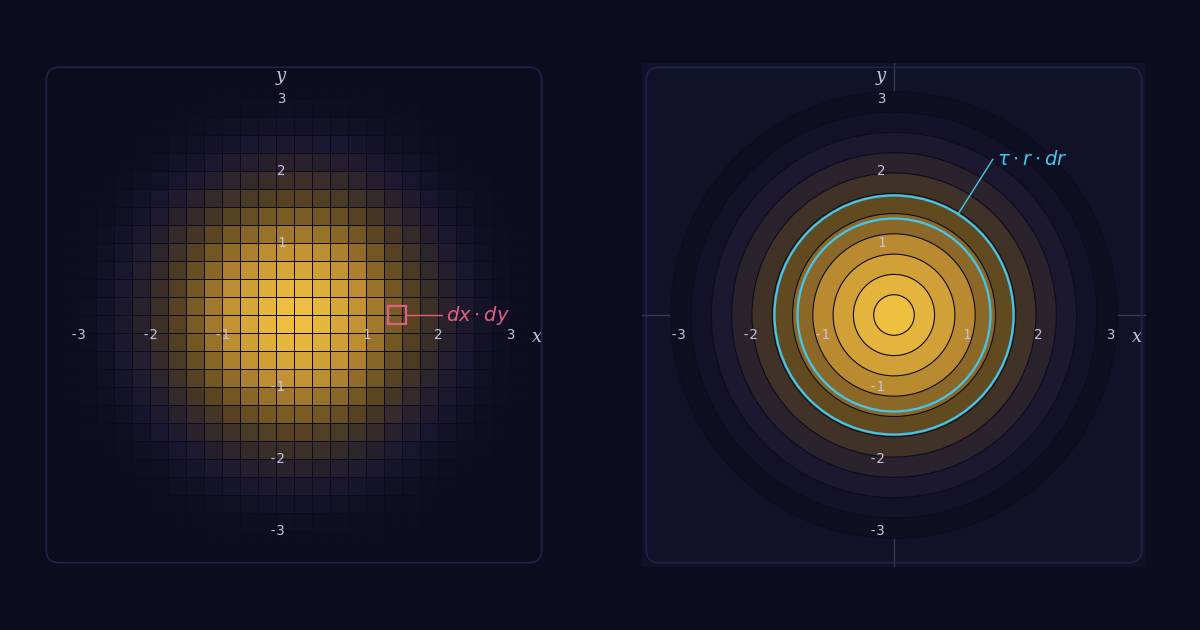
exp(−(x²+y²)/2) as a brightness heatmap: peak at the origin, dark at the tails. Contours at r = 1, 2, 3 are perfect circles — not imposed, but forced by exp's product property acting on two independent straight-line accumulations.
Part 2 — Let the symmetry do the integration
First, read the integral geometrically. The plane is tiled by tiny squares of area dx · dy. At each square, the integrand exp(−r²/2) gives a height (a number between 0 and 1, decided by how far that square sits from the origin). Multiply that height by the square's area, and we have a thin column of volume exp(−r²/2) · dx · dy. The double integral I² is the sum of all those tiny columns over the entire plane — the total volume under the 2D bell surface.
I² = ∑squares exp(−r²/2) · dx · dyNow we can do that sum any way we like, by carving the plane into whatever shapes we choose. The square tiling is one option, but it is not the best one here. Because the integrand depends only on r — every point at the same radius contributes the same height — there is a much more natural carving: thin concentric donuts, one for each radius. Within a single donut the height never varies, so an entire donut becomes a single building block of the sum, replacing many separate squares all carrying the same value.
Square tiling: each tile has area dx · dy and a height exp(−r²/2) that varies from tile to tile.
Donut tiling: each donut has the same height exp(−r²/2) everywhere on it. Same total volume, counted by radius.
Step 1 — the area of one donut. A donut at radius r with thickness dr has area equal to its circumference times its thickness:
area of donut = τ · r · drThis is where τ enters — not as an abstract constant, but as the circumference of the unit circle that every donut inherits.
Step 2 — sum over all donuts. Multiply each donut's area by its (constant) height exp(−r²/2) and add up the contributions. Because every donut shares the same τ, it factors out of the sum:
I² = ∑donuts exp(−r²/2) · τ · r · dr = τ · ∫0∞ r · exp(−r²/2) drStep 3 — what is left inside. Inside the integral sits the function r · exp(−r²/2) — the height at radius r multiplied by the linear circumference factor r. This product has a distinctive shape: near the origin there is plenty of height but very little circumference, so the contribution is small; far from the origin there is plenty of circumference but the height has decayed to nothing. The two effects balance and the curve peaks at r = 1.
The radial integrand r·exp(−r²/2): rises near zero (small donuts), peaks at r = 1, decays in the tail. Total area under it is exactly 1.
Step 4 — the radial integral collapses to 1. Why is that total area exactly 1? Substitute u = r²/2, so du = r · dr. The radial integral becomes a plain exponential decay:
∫0∞ r · exp(−r²/2) dr = ∫0∞ exp(−u) du = −exp(−u) |0∞ = 0 − (−1) = 1A familiar shape returns. The substitution u = r²/2 is exactly §1's natural distance, with r playing the role of time. The factor r in r · dr behaves like a velocity growing linearly with r; u is its triangular accumulation — the very same triangle from §1. So the substitution is not a calculus trick: it is §1's geometry reappearing inside the radial integral, finally delivering the linear factor that exp(−r²/2) has been waiting for.
Putting Steps 2 and 4 together: I² = τ · 1 = τ. Take the square root and the original 1D integral emerges:
∫ exp(−x²/2) dx = √τ ≈ 2.507Total area under exp(−x²/2) is √τ ≈ 2.507. The standard normal probability density is exp(−x²/2) / √τ — not 1/√(2π) — because τ, not π, is the natural constant here.
Part 3 — What we have learned
Look back at the path. We started with the most ordinary one-dimensional thing — x²/2, the natural accumulation of a linear quantity (§1). We found the unique function that bridges additive cost to multiplicative probability — exp, the inverse of the integral of 1/x (§2). We combined them into the bell exp(−x²/2) (§3). And the moment we tried to integrate that bell, a circle dropped out of the sky with its circumference τ attached.
τ was never introduced from outside. It was sitting inside "the integral of x" and "the inverse of the integral of 1/x" all along, dormant in one dimension. The moment a second perpendicular direction was added — and energies and probabilities had to reconcile across it — exp's product property revealed the hidden radial symmetry; the circle carried its circumference τ into the integration; and τ emerged as the exact area under the natural bell. No factors of 2, no bookkeeping, no adjustments.
The Gaussian is not a special function dropped into physics. It is the shape forced on the world by three things at once: a quadratic cost, the multiplicative product rule for independent probabilities, and exp's role as the unique bridge between the two. The constant τ is not a decoration — it is the geometric record of how perpendicular axes combine when energies add and probabilities multiply.
The same calculation with a physical scale K — replacing x with x/√K — gives the general result ∫ exp(−x²/(2K)) dx = √(τK). With K = kBT this is the Maxwell-Boltzmann normalisation; with K = 1 it is the standard normal of statistics. One formula, one constant, one shape — all of them consequences of accumulation, independence, and the geometry of two perpendicular directions.